I am putting my last seminar along with some notes online. This sums up where I stand in my research and what I hope to accomplish in the next eleven months before submitting my thesis.
A few words on the seminar:The Centre for Advanced Spatial Analysis hosts a weekly research seminar. Students are given the opportunity to present their latest results or any form of progress. The slides and notes are part of my third and last seminar - I am also planning to put the first two seminars online. Many of the slides include animations and movies. To view please click on the hyperlinks (blue underline - please allow a few seconds for the video to load). The animations and movies will also be described in the notes. Finally, the notes are somewhat choppy and at times simplistic especially when it comes to reviewing material that was presented in the past seminars. Please feel free to comment and critique.
Slide 1 - Spatial representation & low vision: Two studies on the content and accuracy of mental representations of individuals with a visual impairment or blindness
In my first seminar (over 2 years ago) I discussed the development of spatial knowledge and presented several examples of research on the representation of space by individuals who are sighted, visually impaired and blind. I traced the trajectory from Piaget and his critics to the work conducted by Golledge and others at the Santa Barbara School. I presented results from different studies in Europe with special attention to those conducted by Kitchin, Jacobson & Ungar in the United Kingdom and Thinus-Blanc & Gaunet in France. I presented and explained the three theories described by Fletcher (1980) and argued with some arrogance but I think with enough evidence that the majority of the research conducted in the 90’s worked to fit this three-theory model. Finally, I introduced the re-weighting theory - a more recent and elegant approach to the development of spatial knowledge proposed by Newcombe & Huttenlocher (2003). The seminar concluded with some of the methodological problems related to this type of research.
In my second seminar I introduced the two experiments that I planned to conduct at the Royal London Society for the Blind. I explained how one experiment would test the content and accuracy of mental representation in a known environment while the second would to the same for a new and complex environment. I also mentioned that the second experiment would concentrate on the exploratory strategies used by individuals when faced with an environment for the first time. In the same presentation I discussed the methods I used to collect the data and highlighted the importance of multiple tests when dealing with population that is extremely heterogeneous like the blind and visually impaired. I concluded by framing my approach to Gibson's perception action cycle and phenomenology – By phenomenology I mean the manner in which the individual actively constructs his reality through experience.
In this presentation I will present the results from the first experiment and show how far I’ve got in the second experiment. More important, I plan to convince you of two things: 1-That individuals who are blind or visually impaired are able to construct gestalts of their environment. In other words, that these individuals are able to achieve a configurational (or Euclidean) knowledge of their environment and are able to represent geographic concepts such location, distance, direction and overall configuration. 2-That there is a very important need to recognize and differentiate between ability (possessing the quality to perform) and present competence (the actual performance).
Slide 2 - Structure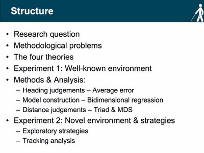 A few words on the structure of the presentation:
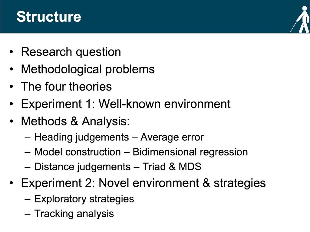
I’ll begin by presenting my research question. Very quickly I’ll go through some of the methodological problems associated with this type research. Next, I’ll review the three theories and introduce a 4th theory – the amodal theory. I’ll then move to the first experiment (the one testing the content and accuracy of mental representation of a well known environment) and present the results for the three tests. I’ll then discuss these results and link them to the second experiment. As I’m still gathering the data, I will explain the rationale for the experiment along with some examples.
Slide 3 - Research Question
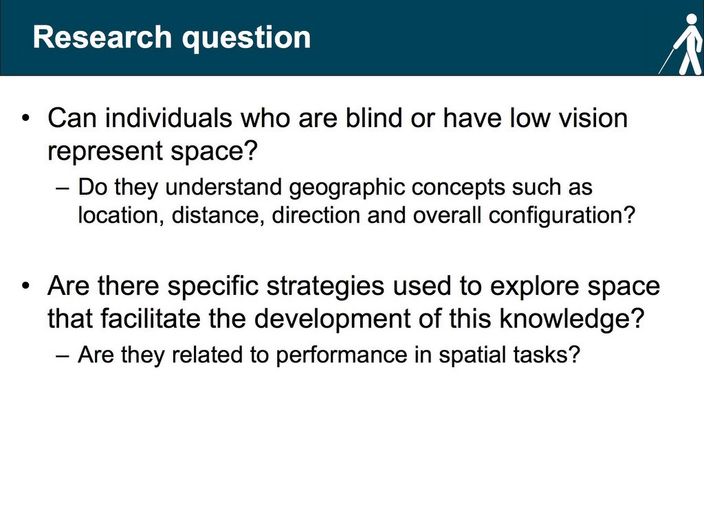
This slide is self-explanatory and presents the two research questions and the rationale for both experiments. The second question is of particular interest as it opens the way for a different approach to understand individual and group (early blind, late blind, mild-moderate VI, severe profound VI & sighted) differences in the development of spatial thought.
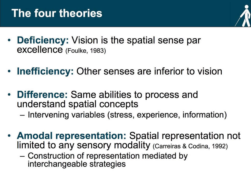
Slide 4 - The four theories
In my first seminar I presented a variety of studies and framed these within the three theories developed by Fletcher (1980). In my second seminar I added another theory by Carreiras & Codina (1992). For now, I’ll just present a quick review of these theories. Details and examples will be available when I put the two other seminars online.
Deficiency: This theory holds that vision is essential for the formation of mental representations. This is an extreme view that has very few supporters and can be said to originate in the work of the German doctor Marius von Senden (1932). After reviewing a series of cases of individuals that recovered from early or congenital blindness (removal of cataracts) von Senden noted that “…the blind can only grasp succession and relation [unable] to produce the completed whole” (von Senden, 1932: p. 288). In other words, vision is the spatial sense par excellence (Foulke, 1983). That is, the early and congenital blind are not able to build overall impressions from fragmentary experiences of the environment collected by the other senses. They are incapable of spatial thought, as they have never experienced the perceptual process necessary to comprehend spatial arrangements. Fletcher (1980) has argued with considerable success that the blind can form gestalts from sequentially perceived information providing evidence from photographs and sculptures by blind artists where different parts of the work are integrated to form a whole.
Inefficiency: The inefficiency theory holds that the other sensory modalities are inferior to vision. That the blind and visually impaired are able to manipulate spatial concepts but that their mental representations are substandard or incomplete when compared to the sighted. Auditory, kinaesthetic and haptic cues are less effective ways of encoding spatial information. Support for this theory is originally found in the work Worchel (1951). Worchel conducted two experiments: The first was a mental matching experiment where congenitally blind (C. blind), adventitiously blind (A. blind) and blindfolded sighted subjects were given two objects (in each of their hand). After feeling and playing with the objects they had to choose (from a set of objects on a table) which object represented a synthesis of the two forms. He found that the performance of the congenitally blind, although above chance, was inferior to that of the adventitiously blind. Moreover, the performance of both blind groups was inferior to that of the sighted. In the second experiment he led subjects along two short legs of a triangle and asked them to return along the hypotenuse. Here again, the sighted performed better than the two blind groups as the congenitally and adventitiously blind made more errors of distance and direction. Echoing the words of Revesz (1933) Worchel denied, “that it should be possible by haptic perception alone to get a homogeneous idea of the form of objects.” There are a series of modern experiments that support this theory and these will be presented when the first seminar is put online.
Difference: The difference theory holds that the spatial abilities of the blind and visually impaired are functionally equivalent to the sighted. They have the same abilities to process and understand spatial concepts but these are developed more slowly and by different means. Jacobson (1997) notes that “lack of vision slows down ontogenic spatial development…but does not prohibit it.” In this manner differences can be explained in terms of intervening variables such as stress, experience and access to information. Juurmaa (1973) notes that one should be careful when interpreting Worchel’s results as these may be flawed and based on a testing artefact. He argues that subjects were dealing with material (triangles or other geometrical forms) that was optically familiar. Differences between groups disappear when asked to synthesize irregular shapes or return to the starting point after being guided through and irregular shaped path. This theory is sustained by the idea that the haptic frame of reference develops more slowly than the visual.
Amodal: This theory will be discussed throughout the presentation and will only briefly presented here. It was first proposed by Carreiras & Codina (1992) and questions the central role of vision in spatial cognition. That is, spatial representation is not limited to any particular sensory modality although processing is probably faster with vision. This theory finds support in work of Susana Millar (1994) as she notes that vision is neither necessary nor sufficient for spatial coding. In her work she presents a theory of overlapping inputs necessary for the coding of space. Finally, this theory allows us approach the construction of mental representations as a result of interchangeable strategies used to explore and understand space.
Slide 5 - Methodological problems
There are a series of methodological problems (more like inconveniences) associated with this type of research and these were discussed in detail in my first seminar. They can be divided in two sections: 1-Problems related to the experimental design. 2-Individual factors.
1-Experimental design1.1-Incompleteness of mental representations: One must be careful when interpreting the absence of phenomena (elements) in mental representations. In perhaps one of the best criticisms of Kevin Lynch’s work, Downs & Stea (1973) note that although many of the subjects failed to account for the John Hancock building it is hard to believe that as Boston residents they did not know about its existence. It is important to differentiate between denotative and connotative meaning. That is, lack of connotative meaning (no significant role) is different from lack of awareness.
1.2-Inferential tasks are more difficult: Tests that require the transformation of an image are harder to complete than tests that involve the recall or recognition (spatial memory) of elements. One should be careful when interpreting and comparing results between different experiments.
1.3-Size of space is an important factor in performance: The layout, size and spatial complexity of the space will produce different results. Some authors (Byrne & Salter, 1983; Dodds et al., 1982) have reported more errors in large spaces while Ochaita & Huertas (1993) argue that performance is mainly a factor of the level of complexity not the size of the space. Again one should be very careful when comparing and generalizing results.
1.4-Size of groups under study: The percentage of the population that is congenitally blind is considerably low (not so much the case for adventitiously blind or visually impaired) and at times statistical tests are performed on small sample sizes. In an extreme case, Spelke (1981) based her results in the performance of one blind subject. Researchers should be encouraged to use larger sample sizes or at least report obvious but essential statistical data such as standard deviations and distributions.
1.5-Numbers of elements to process: Is performance related to spatial ability or to memory and attention? Researchers should differentiate between recall and recognition tasks and be aware of the group’s average capacity (how many?) to mentally store elements. Furthermore, short-term memory suffers from a decay effect that can influence spatial memory tasks. It is important to distinguish the critical times for testing and make sure that all subjects are tested with the same delays.
1.6-Nature of response: Siegel and Cousins (1985) have argued that one should be cautious when interpreting the results from tests that involve an externalization of mental representations. Different tests can generate different results given that the participant’s responses are re-representations of the environment. That is, each type of externalization (verbal, pointing, orienting, sketching, or the construction of models requires specific mental computations that are bound to generate different results (Siegel, 1981). Multiple converging techniques should be used to better understand and interpret results from spatial tests.
1.7-Level of familiarity with the experimental design: Experience can have a considerable effect in the content and accuracy of mental representations. How do we account for the level of experience? When do we consider an environment to be familiar? How do we measure experience with the testing procedure? These are just some of the questions the researcher must take into account before designing the experiment.
1.8-Mode of collection of information: There is a big difference between being the passenger and the driver. Many of us have experienced the awkwardness of getting lost when having to reach a destination visited many times in the past when someone else was driving or guiding us. Experiments should clearly indicate if the collection of spatial information was active or passive (guided vs. free exploration) as this can influence the type and amount of information collected.
2-Individual factors2.1-Type of impairment: Warren (1984) warns about some of the problems when comparing blind, partially sighted and sighted subjects in different spatial tasks. It is hard to classify a population that is extremely heterogeneous. This problems is further complicated given the evidence supporting the variability of individuals with the same eye condition. Individuals can vary in terms of their eye condition, visual acuity and/or field. Some researchers have argued that certain eye conditions have a larger effect on performance. Loomis et al., (1993) found that the performance of individuals with retrolental fibroplasias was significantly inferior when compared to the other VI groups. Dodds et al., (1991) found no such relation.
2.2-Age: What criteria should be used to distinguish the early from the late blind? Researchers from different fields vary in their interpretation of the critical age. For the developmental psychologist it is usually when the infant starts to coordinate movement with vision while for the neuropsychologist this is related to the development of the brain, which reaches its full maturity only after puberty. This has led to different classifications. Rieser (1992) classified as early blind those affected during the first three years, Herman et. al., (1986) until the first year while Millar (1979) before 20 months. In addition, it is important to distinguish static from progressive conditions. This is of particular importance in repetitive or long terms studies.
2.3-Level of education & intelligence: Several studies (Thinus Blanc et al., 1999) have cleverly matched participants in terms of their IQ. Spatial tasks can involve complex mental calculations and performance may be related to the level of education or intelligence.
2.4-Level of orientation and mobility: Many spatial tasks involve learning the location of elements along a route. Good orientation and mobility skills play an important role in the coding and construction of the mental representation. Mobility instructors teach different strategies when walking in familiar and unfamiliar environments and these can prove beneficial during the testing phase.
2.5-Affective development: Confidence and quality of life can also affect performance and researchers should control for the emotional state of the participants. Studies have identified that sudden (accident) or late loss of the visual field is usually associated with depression and difficulties in rehabilitation.
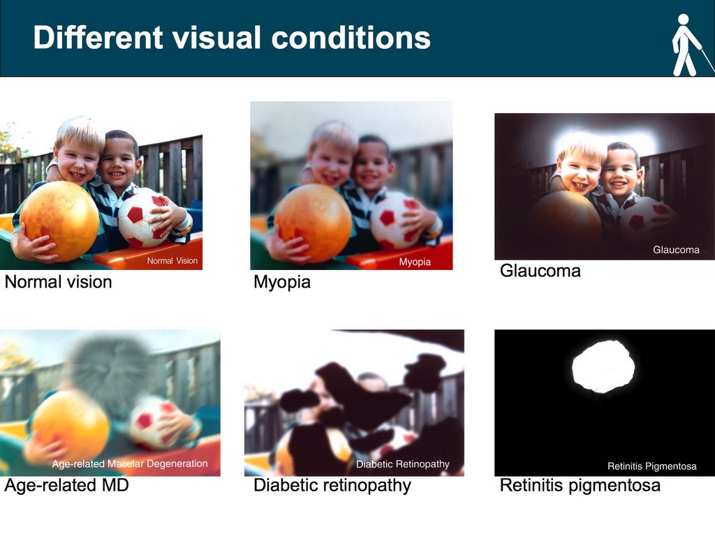
Slide 5.1 - Different visual conditions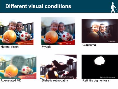
I don’t particularly like this slide as I think it is almost impossible to simulate a visual condition (represent graphically what one can or cannot see). The slide however, allows us to demonstrate that there is a significant difference between conditions and this can lead to considerable problems if all are grouped under a “visually impaired” heading. In a recent working paper I discuss a hypothetical case of two subjects; one with
retinitis pigmentosa (RP) the other with severe
myopia and highlight some of the problems in the testing and classification of these individuals. “Take for example a subject with RP who has poor night vision and happens to be tested during the day. While still impaired due to a restricted visual field (Kanski et al., 2003) chances are that his performance will be significantly different in a situation with low light. How can this individual be put in the same group with someone with severe
myopia whose condition does not significantly vary in relation to lighting changes?” (Schinazi, 2005)
Slide 6 - Experiment 1: Royal London Society for the Blind Campus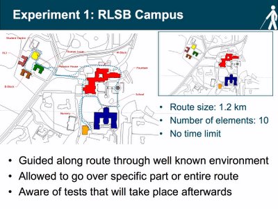
The slide illustrates a simplified model of the
Royal London Society for the Blind campus. This is the setting of the first experiment that will test the content and accuracy of mental representations of a well-known environment. Blind and partially sighted students were guided along a route (blue dotted line) and were asked to remember the location of ten places (8 buildings, 1 fountain and 1 shed). Before walking the route the students were briefed on the research and told what type of tests they should expect to complete. They were also told to think about the actual and relative position between the different places. The testing phase started directly after they finished walking the route.
Slide 6.1 – Visual range
As mentioned above, we are dealing with an extremely heterogeneous population and grouping subjects solely in terms of their visual condition/state can lead to several statistical errors. Researchers should be aware of individual differences and look at different ways to classify visual impairment. In my opinion, a complete study will include different forms of classification (visual acuity, visual field, type of condition and performance) and a discussion of their difference. For the first experiment subjects were classified in terms of their visual acuity. Three groups (mild to moderate visually impaired; severe to profound visually impaired and blind) were created based on a visual range chart proposed by the International Council of Ophthalmology. I am now working to classify these individuals in terms of their actual condition and separate between the congenitally and adventitiously blind. I plan use the same format for the second experiment. In addition, I will introduce a form of classification in terms of performance. This form of classification was first proposed by Hill (1993) and allows for the study of the strategies used to explore space and construct mental representation. I will also argue that this approach allows us to bypass some of the pitfalls related to the heterogeneity of subjects.
Slide 7 – Angle estimation
For the first test students were asked to make pointing judgements using a digital compass. Before the test students were taught how to use the compass and given a few minutes to familiarize themselves with the testing procedure. They were asked to make several pointing judgements (45 in total) from the different locations identified along the route. An accuracy score was generated by calculating the difference between the real and estimated angle.
There has been some discussion as to the relevance or significance of using “absolute error scores” in this type of testing. Montello et al., (1999) note that while it is true that we should also account for constant and variable error, absolute error is probably the best measure of performance, as it requires a low constant and variable error. They argue “one would not consider a person to have high spatial ability if he or she had a large bias (constant error) in pointing to targets but little variability around this biased pointing directions. Nor would a person be considered to have high ability if [the] estimates are always centred on the correct direction but were highly variable.”
An analysis of variance (ANOVA) was conducted and a significant difference in performance was found between the vision groups. A Tukey’s honestly significant difference test (TUKEY HSD) revealed that the difference was between the mild and moderate visually impaired and the blind group (F(2,21) = 5.878, p ≤ 0.009). The three graphs at the bottom of the slide are scatter plots for each vision group. The x-axis represents the real angle and y-axis the group’s estimation. This is just another way of representing the results (goodness of fit). Here we can easily identify a “growing spread” related to the severity of the visual condition.
At first, these results seem to make sense and several researchers have discussed the spatial abilities of the blind and visually impaired based (sometimes solely) on this type of test. However, it is important to note that pointing is not action commonly undertaken by blind people. In my first presentation I discussed in some detail the advantages of vision. For now, it would suffice to say that apart from the ability to quickly form gestalts (wholes) vision allows for the instantaneous collection and assembly of distal information.
Here I would like to go back to what I mentioned in the introduction about the importance to differentiate between ability and present competence. A research that aims to study the spatial abilities of the blind and visually impaired which solely tests individuals in pointing tests does not allow for this distinction. The fact that blind people are not accustomed to point and will have a greater chance of performing at a lower level (greater absolute error) does not mean that the content and accuracy of their representation is substandard. Pointing tests do not allow for the correct externalization of the representation, as blind have different strategies to collect and process distal information. In this manner, a lower performance is related to a testing artefact not the actual spatial ability. This point will be further discussed when the results from the other tests are presented.
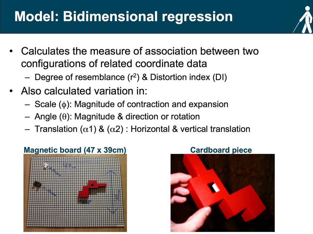
Slide 8 – Model: Bidimensional regression
The next test consisted of building a model of the campus. Model building is an effective way to test for configurational knowledge as it forces the individual to represent the allocentric relationships between the different locations in the campus. Students were asked to complete a cued model. Spatial cued models provide the subject with scale and orientation minimizing the motor skill component. Ten three-dimensional card pieces representing a scaled version of the locations were created. Three were placed on their real cartographic location on a gridded (1cm X 1cm) magnetic white board. Students were asked to position the remaining seven pieces in relation to these.
Results were analyzed using bidimensional regression (Tobler, 1993). A bidimensional regression is essentially a regression for a pair of coordinates. It statistically calculates the degree of association (r2) between two configurations of related coordinate data (Kitchin, 1993). It measures the fidelity in terms of scale (φ), angle (θ) and horizontal & vertical translation (α1 & α2) between where a place is in reality (referent coordinates) and where the subjects thinks it is (variant coordinates). Comparisons are be made by calculating the average r2 for the group. The r2 ranges from 0 to 1 with a higher degree of resemblance as the score approaches 1. Waterman & Gordon (1984) have proposed a distortion index (DI) to measure the overall distortion of the representation after all systematic transformations are performed. Lloyd (1989) notes that this can be thought as a standardized measure of relative error. The distortion index ranges from 0 to 100 (inversely related to r2) and is a dimensionless value. The DI has been substantially reviewed by Friedman & Kohler (2003) who proposed an elegant alternative for calculating distortions without disrupting the relationship between the dependent and independent variables in a regression. The main error associated with Waterman & Gordon (1984) algorithm is that the variants coordinates are always assigned the role of independent variable. For the purpose of this presentation it will suffice to look at the r2 value. A distortion index is still presented but this was calculated with the Friedman & Kohler (2003) algorithm.
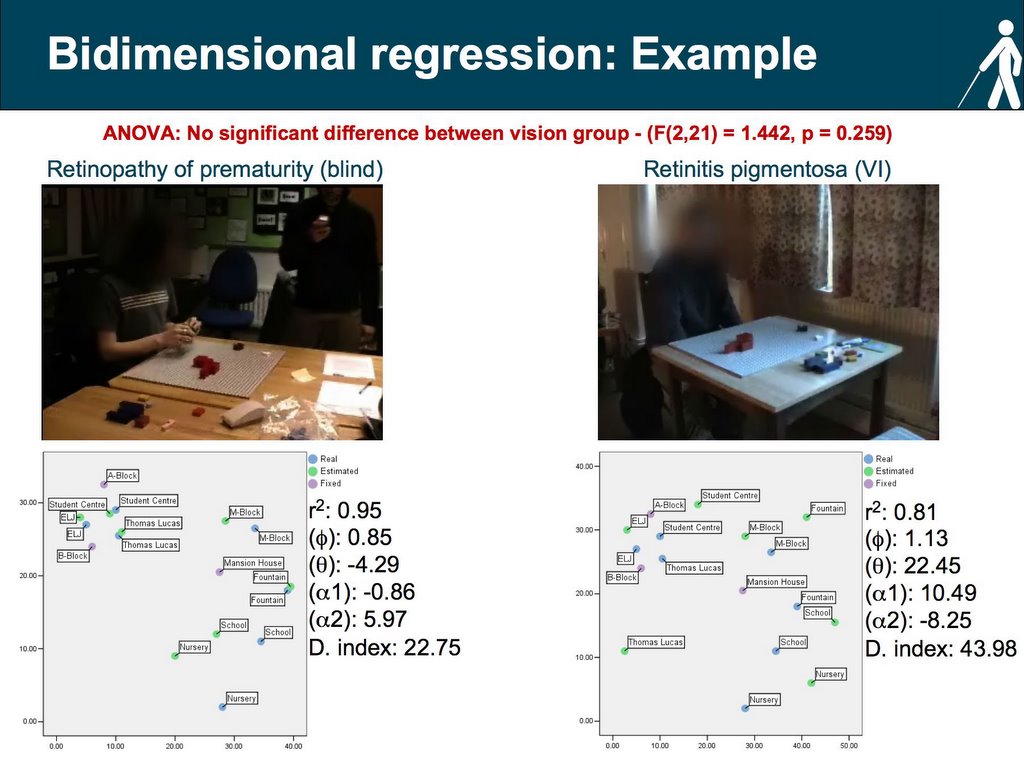
Slide 9 - Bidimensional regression: Example
The slide presents the results of a bidimensional regression for two subjects.
Subject 9 (left) is blind (retinopathy of prematurity) and
subject 16 (right) is part of the mild to moderate visually impaired group (retinitis pigmentosa). Please click on links to open a new window with a video of the subject constructing the model. The performance of both subjects was above chance although the blind subject performed better (r2 closer to 1) than the visually impaired. The graphs below illustrate the position of the real (blue circle), estimated (green circle) and given/fixed (pink circle) of the 10 different locations and allows for a visual representation of the distortion and r2 values. The lists to the right of graphs present the value for the scale, angle and translation changes.
Subjects were divided in three groups (same as in the first test) and an average r2 value was calculated. An analysis of variance (ANOVA) was conducted and no significant difference was found between the three vision groups (F(2,21) = 1.442, p = 0.259). That is, there was no effect of vision in the representation of space when externalized in the form of a cued model. The mean value for the three groups (mild to moderate: 0.68; severe to profound 0.86; blind 0.56) is of particular interest and provides constructive evidence on the ability of this population to represent space. Finally, the outstanding performance of the severe to profound group (average r2 = 0.86) fits with Millar’s (1994) overlapping input theory. That is, these individuals were forced to use to a greater extent a combination of both visual and propioceptive information in order to code space. It is clear that this form of overlap is also present in the other two groups although for the blind and mild visually impaired groups coding may be favoured by a specific modality. In the case of the blind coding is favoured by proprioception while for the mild to moderate visually impaired it is mainly based on vision. We will go back to this discussion when the statistic details of the tests are presented.
Slide 10 – Distance triad: Explained
The last test consisted of estimating distances. Past research has identified that people are not good with exact metrics when asked to make distance estimations. For this reason, a lambda 4 balanced incomplete block design (Burton & Nerlove, 1976) was used to generate a triad questionnaire. This type of data collection has been used with considerable success in the past in similar experiments (Ungar et al., 1996). In this case, subjects were given different sets (60 in total) with three locations visited during the route and asked to estimate which pair of locations is the closest together and which pair is the furthest apart. The questionnaire is scored in the following manner: The pair judged closest is given a score of ”0”, the pair judged furthest a score of “2” and the remaining pair scores “1”. In a lambda 4 design each pair of locations appears four times. This means that the total score for the pair can range from zero to eight. Next, the exact metric Euclidean (straight line) and functional (route) distances are calculated (generated with ArcMap) and using the same questionnaire a score is generated. Errors are calculated by subtracting the estimated from the real scores. In this case you get two error scores (relative to the Euclidean and route metrics). Finally, results from the triad can be arranged into an ordinal matrix of dissimilarities to be mapped and analyzed using multidimensional scaling (MDS). Multidimensional scaling (Jacobson et al., 1995) is a techniques “that allows for a two dimensional representation of a pattern of proximities among a set of locations” (Schinazi, 2005).
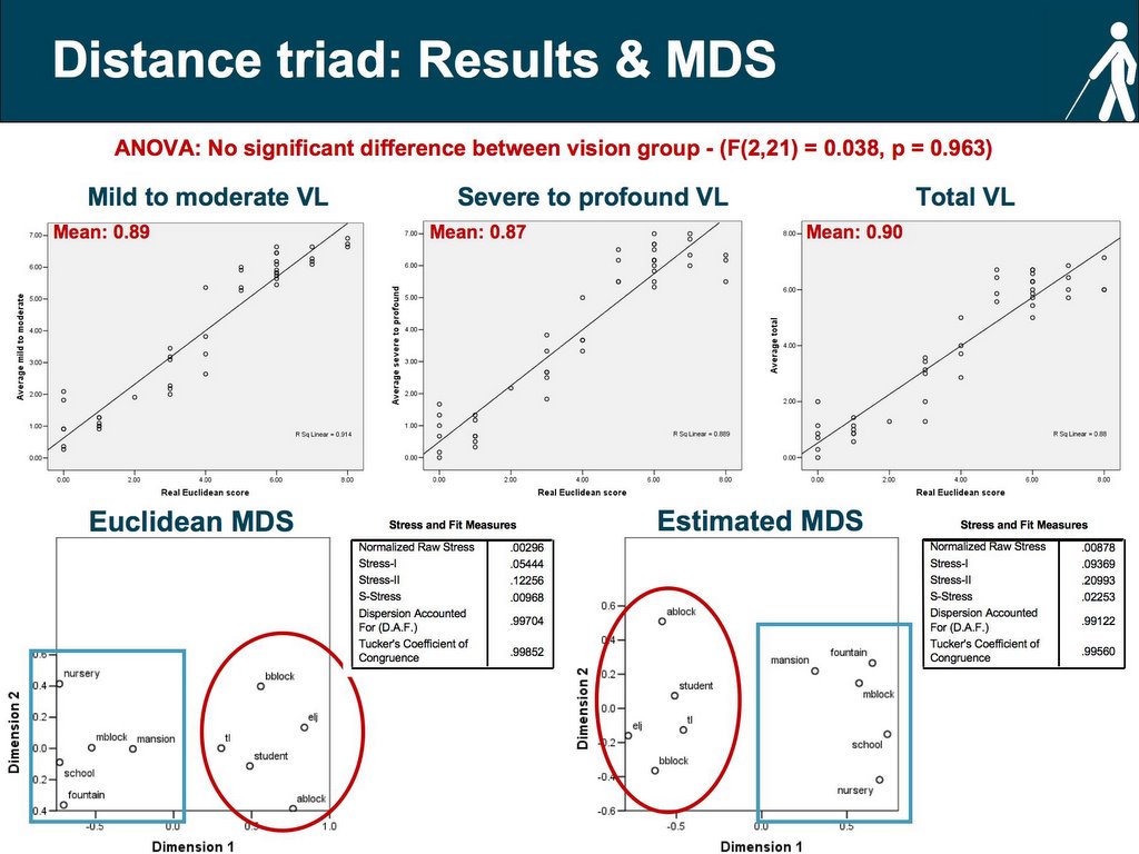
Slide 11 – Distance triad: Results & MDS
An analysis of variance (ANOVA) revealed no effect of vision in the estimation of distances through triadic comparisons (F(2,21) = 0.038, p = 0.963). All groups performed at a relatively high level (mean error - mild to moderate: 0.89; severe to profound: 0.87 & blind: 0.90). As we shall see in the next slide this was the most consistent test across groups with individual errors centred around the mean without any major skews.
The two graphs below are the results of multidimensional scaling derived from the response to the triad questionnaire. Multidimensional scaling allows for the graphical visualisation of a matrix of perceived dissimilarities (see previous slide). The graph on the left is a representation of the location of the ten places visited along the route based on the triad/questionnaire completed with the exact Euclidean metrics. The graph on the right is a representation based on a triad questionnaire completed by a student in the mild to moderate visually impaired group. The two tables next to the graphs present the stress values for the scaling.
The main problem with MDS is that it is very hard to compare representations (graphs). This is because the MDS algorithm is concerned only with the relative proximities between the different elements (in our case the ten locations visited along the route) and does not account for their absolute position in space. What it does provide however, is useful information for a typological type of analysis as it is able to illustrate groups or clusters of locations. If you scroll back to the map of the RLSB campus (slide 6) you’ll notice that the campus can be divided in two sections: 1-The college area includes A-block, B-Block, Student Centre, Thomas Lucas and ELJ. 2-The school area includes the Mansion House, Nursery, School, Fountain and M-block. These two clusters can be seen in the Euclidean MDS (college area = red circle & school area = blue square). The same clusters can also be seen in the MDS derived from the triad questionnaire completed by a subject from the mild to moderate group.
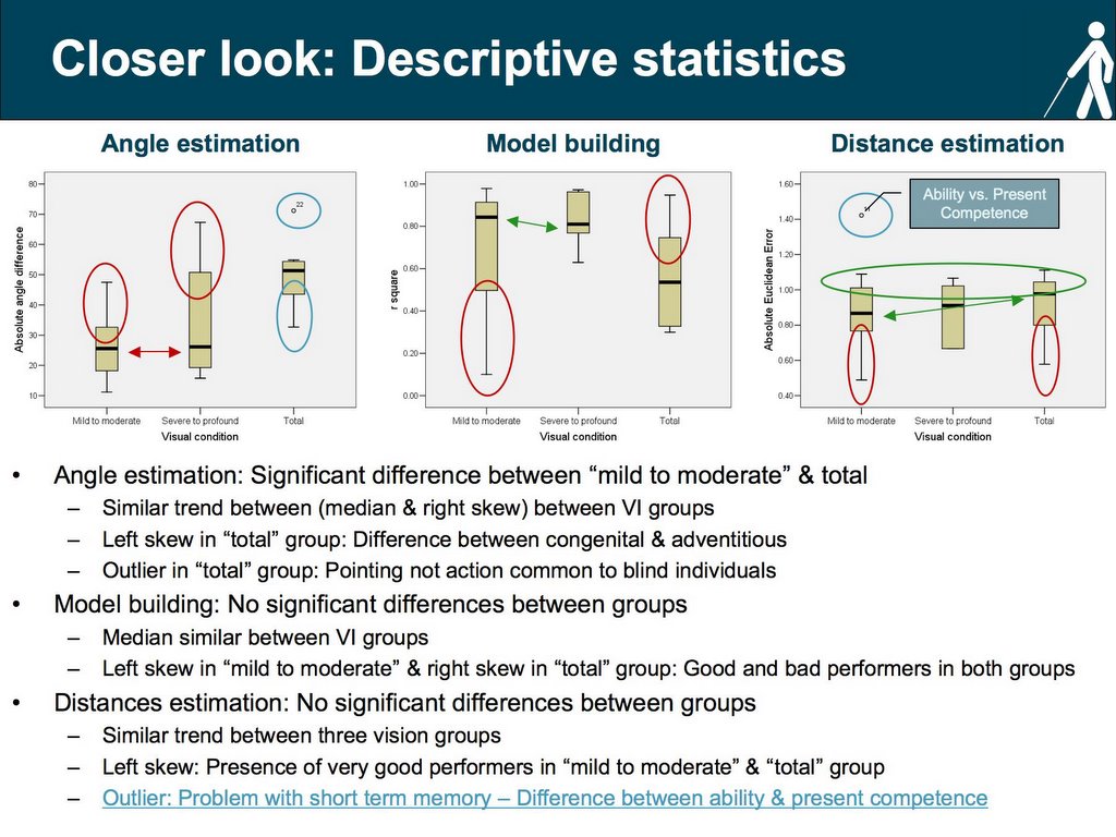
Slide 12 – Closer look: Descriptive statistics
This slide is an essential part of my research as it links the two experiments conducted at the Royal London Society for the Blind. It is basically an analysis of the descriptive statistics for the three tests that were conducted. More important, it provides convincing evidence for the presence of good and bad performers in each group.
A few words on box plotsBox plots are an efficient method of displaying different aspects of a distribution (Tukey, 1977). They provide a “visual summary” of the median, upper/lower quartiles and minimum/maximum data values and are of particular interest when viewed side by side and used to compare data from different groups. The median (the middle of the distribution) is the line that runs across the box. The box itself stretches from the lower hinge (25th percentile) to the upper hinge (75th percentile). The lines that stretch out of the box are known as whiskers and they indicate the minimum and maximum data values. Points located beyond the whiskers (on either side) are called outliers. If the median line is not equidistant from both hinges the distribution is skewed. In a positive (right) skewed distribution the mean is larger than the median. In a negative (left) skewed distribution the mean is smaller than the median.
1-Angles estimation: If we look at the first box plot we are able to identify several important differences/similarities in the distribution of the three vision groups:
The median for the two visually impaired groups is about the same. Although there is a noticeable right skew in the “severe to profound” group there was no effect of vision in the estimation of angles for these two groups. A significant difference was found between the mild to moderate and the blind group. Looking at relatively high mean and median of the blind distribution, it can be argued that the positive skew (decline in performance) is a reflection of an effect of vision or as argued before the result of testing artefact that favours vision. The right skew also points to a considerable presence of bad performers in the “severe to moderate” group. Further analysis will determine if there is a relation between the level of performance and the type and age of onset impairment. Finally, given that there was no significant difference between the two visually impaired groups for this test (as we shall see the same is true for all tests) it can be argued that they are part of the same population and can be grouped (this will be done at a later stage) to form a mild to profound visually impaired group.
If we look at the box plot for the blind group the situation is reversed. Here we see a high median (high absolute error) with the vast majority of individuals performing at a low level. Moreover, while the distribution is negatively skewed pointing to the presence of a few good performers, the minimum whisker is still above the median for both vision groups. In this case a relation was found between performance and the age of onset blindness. Finally, we also note the presence of an outlier (subject # 22). It is worth noting that in the box plots for the other tests (model building & distance estimation) this subject falls within the distribution. This provides further evidence for the ability and present competence debate.
2-Model construction: In the box plot for the model construction test one can easily notice that although there was no effect of vision in the construction of the model, the distribution for the three groups is considerably different.
The box plots point to the presence of good and bad performers in the three groups. This type of data needs to be approached and analysed within the “individual differences” paradigm. This paradigm accommodates an amodal interpretation (vision neither necessary nor sufficient for spatial coding) of the data. The main objective lies in the identification/isolation of the reason behind the variability in performance within each group. In other words, what is causing some people to perform better (in some cases – much better) than others? We will get to this in the following slides – for now let us concentrate on remaining characteristics of the distributions in the model construction test.
Looking at the box plot for the “mild to moderate group” we note that it houses the best and worst performers for all three groups (look at high and low whiskers). Although the median is relatively high the left skew (group mean lower than the median) points to a considerable presence of bad performers. In the “severe to profound” group we note that although the median is slightly lower when compared to the “mild to moderate group” the distribution is characterized by a positive skew (mean larger than the median). Overall, this is the best performing of the three groups where even the lowest performer (lower whisker) falls well within the distribution of the two other groups. The box plot for the blind group shows a normal distribution (median and mean about the same). However, when compared to the two other vision groups, the 25th percentile of the distribution is the lowest and the 75th percentile falls below the median of the two other groups. At the same time, the high whisker points the presence of a very good performer.
3-Distance estimation: The box plots for the distance estimation task shows a similar trend for the three vision groups. In this case, the median for the three groups is relatively the same and although the three distributions are skewed the mean and median disparity is not as acute as in the other cases. Although the best performer is in the “mild to moderate group” (low whisker), the negative skew in the “severe to profound” and “blind” groups point to the presence of good performers. It is also worth noting the presence of a very good performer in the blind group. As mentioned before, this is the test where overall performance (3 groups) was the highest (even if some subjects reported that this was the hardest test to complete).
What is the reason behind this good performance? I would like to argue that when completing the distance questionnaire subjects make use of a temporal dimension, which if not present is at least not as evident in the two other tests. That is, responses are weighted in terms of vision (in the case of the sighted or VI), proprioception (sighted, VI & blind) and a temporal element (how much time did it take to get from point A to point B). It is the combination of these 2 (sometimes 3) inputs, an overlap of cognitive dimensions, which facilitates estimations and provides more accurate answers.
Finally, we notice the presence of an outlier (subject 11) above the high whisker of the “mild to moderate” group. This brings me back to the ability and present competence debate (and the beauty of collecting ethnographic type data). A closer analysis of the video of this subject answering the distance questionnaire revealed that the subject experienced considerable difficulties when having to simultaneously retain the names of the three locations. While this subject’s performance in the previous tests was within the group mean both tasks did not require a constant referral to short term memory. The tests were conducted in a well-known environment and involved to a larger extent the use of and already internalized (long-term) representation. The distance estimation test also required the use of this internalized representation; however, the fact that it was verbally administered forced the subject to multi-task between short and long term memory.
Slide 12.1 – Ability vs. present competence
To conclude on the ability and present competence discussion two other tests were conducted:
1-Ranking: The scores of the different participants for the three tests were ranked. The bar graph indicates how subjects ranked differently (sometimes considerably different) depending on the task and highlights the need of multiple tests when comparing performance. In the following months, I plan to conduct a series of non-parametric tests in order to ascertain the significance of this relationship.
2-Test difficulty: Subjects were asked to choose which test they considered the hardest to complete. A chi-square test revealed that there was no preference among groups for any specific test (χ2 = 1.974, df = 4, p = .741). In other words, there was no agreement between groups as to the difficulty of the different tests. That is, what one subject in a particular group considered as an easy task was not always the case for the rest of the group.
Slide 13 – Explaining the difference: Mobility & LVQOL
The difference in performance between individuals in the same group (in the three tests) leads us to one very important question: What is causing some of the subjects in each group to perform better than others? As a complement to the collected data, subjects were asked to respond to two additional questionnaires.
Mobility Questionnaire: The aim of this questionnaire is to assess the level of orientation and mobility of the participants. Participants were presented with fifteen different mobility situations and asked to rate on a scale from 1 to 5 the amount of difficulty experienced in a particular situation. This questionnaire is an adapted version (used with permission) of Turano et al., (1999) independent mobility questionnaire for individuals with retinitis pigmentosa. Full reference: Turano, K., Geruschat, D., Stahl, J., & Massof, R. (1999). Perceived visual ability for independent mobility in persons with retinitis pigmentosa. Investigative Ophthalmology & Visual Science, 40, 5, 865-877.
Quality of life questionnaire: The aim of this questionnaire is to measure the quality of life of individuals with low vision. The questionnaire is divided into four parts: 1-Vision mobility & lighting; 2-Psychological adjustment; 3-Reading & fine work; 4-Activities of daily living. Participants were given different situations and asked to rate their ability to cope with it. This questionnaire is an adapted version of Wolffsohn & Cochrane (2000) LVQOL. Full reference: Wolffsohn, J., & Cochrane, A. (2000). Design of the low vision quality of life questionnaire (LVQOL) and measuring the outcome of low vision rehabilitation. American Journal of Ophthalmology, 130, 6, 793-802. Blind subjects only completed selected items of this questionnaire as it is designed to assess quality of life of people with low-vision.
The questionnaires were given to a teenage population with little previous experience with rating scales and it was important to check for some sort of consistency in response. A significant correlation was found between the mobility and quality of life scores (r = 0.844, n = 21, p ≤ 0.001). Here it is important to note that the quality of life questionnaire incorporated several questions that dealt with mobility aspects of everyday life (the minus sign next to the correlation “r” is because the scales in the questionnaires are reversed).
No difference was found in the level of independent mobility between the three vision groups. More important however, is the relation between the level of independent mobility and quality of life (2 questionnaires) and performance in the three tasks. The table in the slide shows the correlation coefficient for the visually impaired group (groups gathered: moderate to profound) between performance in the three tasks and the questionnaire scores. Results indicate the existence of such correlation (in some cases very significant). That is, good performers also had a positive rating in the mobility and quality of life questionnaire.
This is when is starts to get interesting...The same correlation test (between performance and level of independent mobility) was performed for the blind group and no significant relationships were found. These results may seem somewhat puzzling especially if we consider that there was no difference between groups in their level of independent mobility. There are however, two possible answers to this problem: First, given these subjects were tested in a well-known environment it can be argued that the individuals in the blind group reached some sort of mobility threshold. This threshold should be understood in terms of an aid but not an effect in task completion. The second answer is that there may be something else influencing the performance of these three groups. For the remainder of the presentation I will argue that a very important factor in task performance is the manner in which these individuals construct and code space. This will be approach by a study of the strategies used when exploring a novel environment. Finally, it is worth noting that gender did not have an effect in performance. Results of a t-test conducted for the three tasks yielded no significant results.
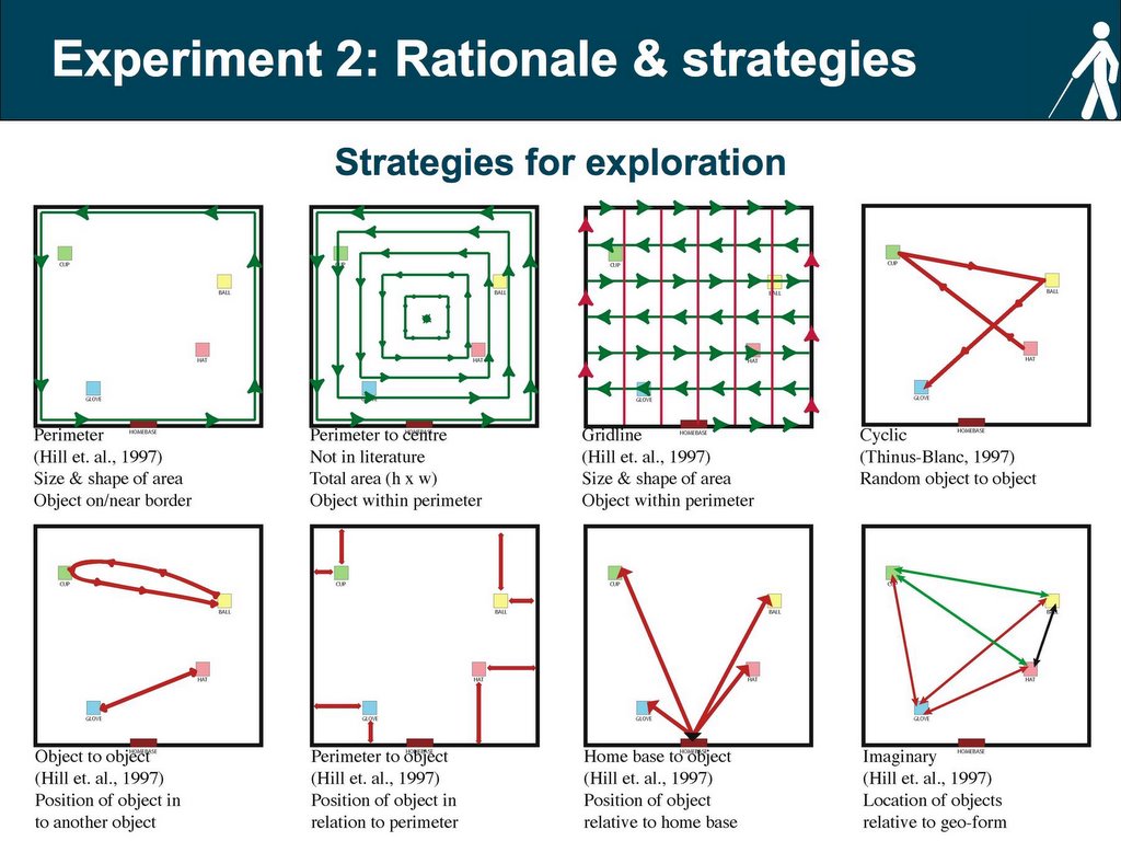
Slide 14 – Experiment 2: Rationale & strategies
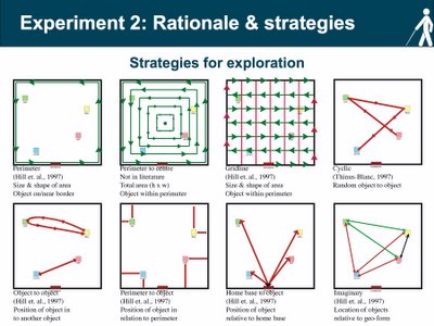
Research on exploratory strategies is relatively scarce with a few notable exceptions (Hill et al., 1993; Thinus-Blanc & Gaunet, 1999). Nonetheless, orientation and mobility has identified a series of strategies used by individuals when exploring space. For the moment it is important to differentiate between two types of spatial coding. A person can code the location of an object in space in terms of their body (egocentric coding) or in relation to other objects in space (allocentric coding). Like the development of route to configurational knowledge (Siegel & White, 1975) some researchers have argued that spatial coding develops from egocentric to allocentric. There is substantial debate as to the validity of both these progressions. If we look at the strategies schemas above we note that some are egocentric (perimeter, gridline) while others are allocentric (object to object, perimeter to object). The main idea behind the study of strategies is to investigate whether there is a relationship between the strategies used to explore and code space (of a novel environment) and the level of performance in different spatial tasks. A full description of the strategies will be posted in the following weeks along with the slides of the 2nd presentation.
Slide 15 – The maze

A maze was constructed at the site of the Royal London Society for the Blind (RLSB) in Sevenoaks, Kent. The maze is a network of barrier fences mounted on wooden poles and consists of corridors, open spaces and dead ends. Inside the maze there are 6 tables, these are labelled (large card signs & Braille) and represent six different locations in an imaginary city: coffee shop, train station, school, bakery, police station & bank. The
video on the left is an accurate walkthrough animation of the maze. The
video on the right is a walkthrough of the actual maze.
The subject is brought to the entrance (told that the entrance is the same as the exit) and asked to explore the maze, locate and remember the position of the six different tables. Unlike the previous experiment, exploration is not guided. Subjects are given a maximum time of 45 minutes and told that the researcher would follow behind with a video camera in order to capture their search pattern.
The majority of subjects took part in the first experiment and were told that they would be tested in the same manner. That is, they would be asked to make heading judgements, to complete a cued model and estimate distances. In addition, subjects were asked to complete a utility task. Here the subject is asked to visit in a specific order and by the shortest route four different locations (tables) in the maze. This type of test also requires an externalization of a mental representation. However, unlike the previous tests, it involves action in the real environment.
I have already collected the data for 27 subjects and I am in the process of entering and analysing it. The first part of the analysis will be much like the one presented in the previous slides. I will also take the opportunity to make comparisons between performance in a known and novel environment. For the second part of the analysis, I plan to relate performance on the four tests to the different strategies the individuals used to explore space.
Slide 15.1 – Maze photos
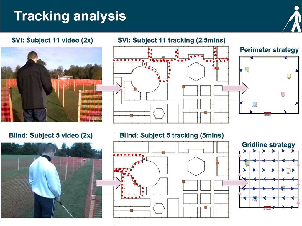
 Slide 16 – Tracking analysis

I am currently working on the details of the analysis. For now, the idea is to divide the exploratory patterns into different time sections and isolate the strategy or strategies used during the different sections. The patterns will be entered into ArcMap using tracking analyst. Once all the data is entered the different type of spatial patterns will be extracted and combined with the known strategies into a data match questionnaire. The idea behind the questionnaire is to match the spatial patterns made by the subjects to a list of possible strategies that were previously identified. The questionnaire will inevitably be very long and for this reason it will only be given only to a selected panel. The panel will consist of experts in the field of blindness and visual impairment and it will range from orientation and mobility instructors, teachers and life-skills tutors. Inter annotator-agreement (inter-rater reliability) will be assessed with Cohen’s Kappa. Next, a table will be constructed that will contain each subject and the type and frequency of strategies used. The final analysis will consist of matching the frequency and type of strategies to performance in the four spatial tasks.
The video on the top left corner shows a section of the maze exploration by a subject in the “severe to profound” group. The two figures to the right present the progression of the analysis. The first figure is that of the search pattern coded in ArcMap the next figure shows the perimeter strategy that matches it. Below is another example for a subject in the blind group. Here the subject made use of the gridline strategy.
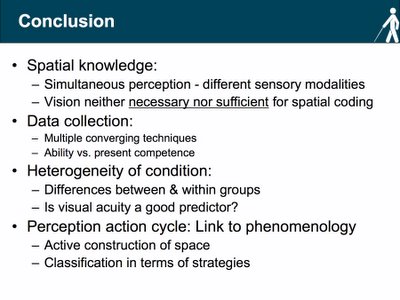
Slide 17 - Conclusion