It is amazing that in the third year of my Ph.D. I find myself home on a Saturday evening (yes, I know what an exciting social life) writing about statistics. Yet, I have spent the past few days reviewing several articles in geography and psychology on the representation of space without vision that have relied on inferential statistics in the presentation and interpretation of results. These have not been pleasant days to say the least as some researchers continue to employ a variety of methods without a clear understanding of their purpose and meaning. More often than not, the probability values (p values) in null hypothesis significance testing (NHST) are misinterpreted which inevitably lead to false conclusions about the data. It was not long before I realised that a review of NHST was in order. During the past two decades, NHST has been under severe criticism. My goal is to present a brief review of this more than justified critique and discuss a variety of complimentary methods. This is by no means an in depth review and I suggest that anyone conducting this type analysis have a look at the list of books and articles below. While you are at the library it would probably not hurt to pop in the mathematics section and browse thorough John Tukey’s book
Exploratory data analysis. As we shall see, the majority of the methods that should be used as either an alternative or complement to NHST are derived from Tukey’s work.
Chatfield, C. (1985). "The initial examination of data." Journal of the Royal Statistical Society. Series A (General) 148(3): 214-253.Cohen, J. (1990). "Things I have learned (so far)." American Psychologist 45(12): 1304-1312.Cohen, J. (1994). "The earth is round (p <.05)." American Psychologist 49(12): 997-1003.Coe, R. (2000). What is an 'Effect Size'? University of Durham. 2000. http://www.cemcentre.org/ebeuk/research/effectsize/ESguide.htmKline, R. B. (2004). Beyond significance testing: Reforming data analysis methods in behavioral research. Washington, DC, American Psychological Association.Schmidt, F. (1996). "Statistical significance testing and cumulative knowledge in psychology: Implications for training of researchers." Psychological Methods 1(2): 115-129.Smith, F. A. and A. D. Prentice (1993). Exploratory data analysis. A handbook for data analysis in the behavioural sciences: Statistical issues. G. Keren and C. Lewis. Hillsdale, New Jersey, Lawrence Erlbaum Associates Publishers: 349-390.Wainer, H. and D. Thissen (1993). Graphical data analysis. A handbook for data analysis in the behaviour sciences: Statistical issues. G. Keren and C. Lewis. Hillsdale, New Jersey, Lawrence Erlbaum Associates Publishers: 391-458.Tukey, J. W. (1977). Exploratory data analysis. Reading, Mass.; Don Mills, Ont., Addison-Wesley Pub. Co.
So why am I doing this?
I would like to think that I am not stating the obvious but rather what should be obvious. When preparing this manuscript I could not help but wonder whether it really is a necessary part of my research. After all, a review of statistics seems like fairly basic material to cover in a doctorate thesis. It was not long before I discovered that many articles on blindness and visual impairment published in academic journals in geography and psychology have not taken into account some of the dangerous limitations of NHST and the noteworthy alternatives that have been proposed.
These disciplines have a long tradition of comparing between different groups of participants. Much of the research has focused on the way in which individuals within a group are similar to one another but different from other groups. In this case, comparing the abilities to mentally represent space of the sighted in relation to the visually impaired and blind. Conversely, very little attention has been paid to the ways in which individuals within a specific group differ from one another (Lewis & Collis, 1997). Comparing the abilities between individuals in different groups can provide important information on the role of vision in the representation of space and can assist in the formulation of theories on sensory substitution and proprioception. At times however, this method of comparison can be problematic especially when the adopted methodology does not allow for individuals in a specific group to fully express their abilities. This is often the case in experiments that compare the performance of blind and visually impaired subjects against a blindfolded control. In such cases the blindfolded control usually operates at a disadvantage as they are forced to rely in different strategies to problem solve. Similar problems occur in research that uses fully sighted controls. In many cases, the type and amount of information provided by the researcher for the completion of a specific spatial task tends to vary between groups. In this manner, Millar (1997; 2000) argues that performance is not based on actual spatial competencies but differences in the provision and access to the information that is necessary to complete the task. Finally, comparative approach does not offer the researcher any insight on the underlying processes that make up behaviour and influence these abilities.
The phenomenological world of the visually impaired is qualitatively different from that of the sighted (Rosa, 1993). If the two years I have spent working at the Royal London Society for the Blind have taught me anything is that individuals with visual impairments and blindness form part of a population that is extremely heterogeneous that many times cannot (and should not!) be classified in specific groups or categories. The tradition of making comparisons between groups assumes that individuals that make up a particular group share the same characteristics. In the majority of cases people with visual impairments are often grouped together because they have been diagnosed with the same eye or medical condition, share the same aetiology or because they have performed at a specific level in psychometric tests. Unfortunately, these types of classification are somewhat restrictive. Consider the case of individuals who are diagnosed with the closest matched condition. In such cases the expert does not know the exact nature of the impairment and bases his diagnostic on the present manifestation of symptoms and behaviours. Some of my students have been diagnosed with a specific condition (most of the time retinitis pigmentosa) although they do not exhibit many of the characteristics that the condition incurs. This type of unforced professional error cannot account for latent behaviours or symptoms and may cause a significant amount confusion if these individuals are mixed together in the same group. The fact the retinitis pigmentosa is a degenerative condition further complicates matters.
The lack of vision cannot fully account for the differences. Such strict causality is theoretically sterile (Warren, 1994) and does not recognize the growing amount of evidence on the spatial abilities of the blind and visually impaired. While the nature and history of the condition can have important implications for the development of spatial understanding concentrating on the pathology of the impairment is clearly not enough. The development of spatial abilities is also mediated through interaction and experience with the environment and culture. In this manner, while the group may be similar in either a medical, functional or clinical diagnosis (or any combination of these) is still not entirely homogenous. The comparative approach can be beneficial if the researcher is capable to control for a certain amount of cohesion within each specific group. This method is better suited when large and clear differences exist. However, when differences are slight or inexistent a differential or individual differences approach may be more suitable.
The individual differences approach accounts for the variety of effects that different factors and conditions have on the specific individual (Lewis, 1993). It focuses on two questions that cannot be fully explained by the comparative method. First, what is the nature of the variation? Second, what are the causes leading to such variation? Research on visual impairment and blindness is filled contradictions and it is not uncommon to find similar studies with conflicting results. In this manner, the first and a crucial step of this approach is to provide a detailed description of the characteristics of the group and each participant as an individual. Many discrepancies between studies can often be attributed to the fact that researchers were working with samples that were not equivalent (Warren, 1984). The second step consists of identifying the correlates and the reason and cause(s) for the variation. The individual differences approach combines the logic of the case study technique with the advantages of quantitative methods.
There are several difficulties associated with this approach and these are mainly related to vast array of factors (physical, clinical and environmental) that even if identified can have a different effect on each participant. However, it is exactly this complexity that should interest researchers. Good research is the one that not only identifies the statistical significance of an effect but also the magnitude and reasons that can explain it. Explaining the difference is what will aid professionals in the design of intervening programs that are catered to the group or the specific individual.
How does this relate to null hypothesis testing?
In the final chapter of his seminal book Blindness and early childhood development David Warren (1984) expresses his disappointment about the quality of past research. This dissatisfaction stems mainly from methodological and analytical weaknesses that fail to account for the heterogeneity of the population. Researchers often overlook the need for detailed descriptions of the various characteristics of the population. In fact, the attention that should be ascribed to these descriptive techniques is usually forfeited in exchange for statistical significance testing that more often that cannot provide any explanation regarding the presence of an effect. Perhaps the most obvious reason behind the ineffectiveness of NHST is the fact that the tests most commonly used (Student’s t-test and Analysis of variance) rely on group averages (mean) and are based on the assumption of a normal distribution. An analysis solely based on group means is unrealistic and short sighted. Researchers studying visual impairment and blindness cannot afford to “indulge in the luxury” of studying only group means and disregard any variations from it (Warren, 1984, p. 298). A certain amount of variability will always exist and some reasons can almost certainly be traced to determinant factors. It is the duty of the researcher to record and report these characteristics and make the necessary efforts to explain the presence/absence of an effect not only for the group but for subgroups or specific subjects that do not follow the trend.
The history of psychology is filled with examples of renowned researchers (Piaget, Vygotski) that have managed to reach important conclusions without relying on significance testing. Unfortunately, many are still under the illusion that results accompanied by significant probabilities values (p values) are more robust and a fundamental requirement for publication. As we shall see, the null hypothesis is always false and rejecting it is only a matter of securing a large enough sample. In addition, results that are not statistically significant should also be considered and reported. Not finding an effect (or a difference) can provide relevant information about the reliability and adequacy of the chosen methods and can lead to a reassessment of the entire experimental design. Results that fall short of statistical significance will also force the researcher to consider the other array of “self selected” or “status” variables that are brought by each individual participant and are beyond the control of the experimenter.
We are now faced with an important and yet somewhat paradoxical question. If the need to change from a comparative (or at least include) to an individual differences approach was identified in the early 80’s why have so many researchers failed to incorporate this in their research design? Why after having identified serious problems with NHST do researchers continue to rely exclusively on statistical significance to explain their results?
The problems with NHST
The problems associated with NHST are not new. In fact they have been around for so long that one cannot help but feel ashamed that for past two decades a considerable amount of research has been conducted (hypotheses have been tested) under such an inadequate and insufficient system. A recent article on the Economist (January 2004) criticizes the over reliance on statistical significance testing rather than logical reasoning on the part of social scientists. It denounces the misuse of statistical data and argues that more often than not researchers do a lousy job when manipulating and making sense of numbers. The wide availability of computers and the ease of use of several sophisticated statistical packages have fuelled a bogus statistical revolution whose main order is to test for significance. Statistics can be deceptive especially when they are used to explain human behaviour. Significance testing does not tell us whether differences actually matter or provide any explanations. The researcher’s dependency on significance testing has lead to variety of problems especially when these have failed to separate statistical significance from plausible explanation.
Despite years of ferocious criticism and recent guidelines published by the American Psychological Association (APA) many researchers in geography and psychology continue to use NHST to interpret and explain their results. Perhaps the biggest problem stems form the fact that there is lack of comprehension regarding the concept of statistical significance. Results from significance tests can be somewhat deceptive at times giving the illusion of objectivity and it is important that researchers understand the purpose and implications of these tests before applying them. Cohen (1994) points to three common mistakes frequently made by researchers: 1-The misinterpretation of p as the probability that the null hypothesis is false. 2-That when we reject the null hypothesis p is the probability of successful replication. 3-That rejecting the null hypothesis affirms the theory that led to the test. More recently, Kline (2004) has outlined several false conclusions that derive from these misinterpretations. These authors among several others (Chatfield, 1985; Schmidt, 1996; Smith & Prentice, 1996) have put forward a variety of methods such effect size measures, confidence intervals, point estimates that combined with graphical tools that can be used as a replacement or complement to NHST. Before we can review these methods and critiques we must first clarify the purpose of NHST. What does the p value really tells us? And what can we conclude when a result is said to be statistically significant and we can reject the null hypothesis.
NHST indicates the probability (p) of data (or more extreme data) given the null hypothesis is true. The p value is a probability statement. It is the measured probability of a difference occurring by chance given that the null hypothesis is actually true. In other words it measures the strength of evidence for either accepting or rejecting the null hypothesis. A small p value suggests that the null hypothesis is unlikely to be true. It does not tell us the probability that the null hypothesis is false. Clearly these are two different things. However, much research has been conducted under the illusion that the level of significance in which the null hypothesis is rejected (usually .05) is the probability of its veracity (Cohen, 1994). The verity of the null hypothesis can only be ascertained through Bayesian or other type of statistics where the probability is relative to the degree of belief and not frequency (Cohen, 1990).
The six fallacies
As Cohen (1990) has impeccably noted, what researchers would like to know is how likely there are differences in the population given the data. Unfortunately all that NHST can provide is information on how likely is the data, given the assumption that there are no differences in the population. The list below is an adapted version of Kline’s (2004) review of the typical false conclusions adopted by researchers who misinterpret the meaning of the value of p in NHST:
Magnitude fallacy: This is the false belief that the p value is a numerical index of the magnitude of an effect (strength of the relationship). That is, the lower the p value the larger the effect. Psychology and geography journals are filled with examples that deliberately regard a difference at (.001) level as more important than one at the (.05). These are wrong interpretations given that the p value only indicates the conditional probability of the data given that the null hypothesis is true. Significance levels are highly dependent on sample sizes to the point that “highly significant differences in large sample studies may be smaller than even non-significant differences in small sample studies” (Schmidt, 1996, p. 125). Increasing the sample size will almost always lead to results that are statistically significant. As we shall see, the effect size is what tells us about the magnitude of an effect - strength of the relationship between the independent and dependent variables.
Meaningfulness/causality fallacies: The false belief that rejecting the null hypothesis automatically asserts the truth (proves) of the alternative hypothesis. Rejecting the null hypothesis does not imply a causal relation. The alternative hypothesis is only one of many possible hypotheses and rejecting the null hypothesis does not confer exclusivity to a specific theory. There are may be a variety of possible intervening and yet to be identified factors not covered by the alternative hypothesis. Replication is perhaps the best evidence.
Failure/quality fallacies: The wrong conclusion that if you do not reach significance at least at the (.05) level (if the null hypothesis is not rejected) than the study is a failure. In other words, reaching significance is what dictates the quality of the study. Type II errors can occur when statistical power is low or the overall research design and methods are inaccurate. Failure to reject the null hypothesis can be an important part of the research. It forces the researcher to look for the reasons behind this lack of difference/significance and allows for a critique of the actual data and methods. In some cases, failure to reject the null hypothesis along with a well-sustained explanation of the data will raise questions about the validity of past research.
Sanctification fallacy: This is related to the failure/quality fallacies and deals with the fact that many researchers credit a finding as significant if it falls between the sanctified (.05) and (.01) level but consider the difference or relation insignificant if the value of p is larger, even if only marginally larger. As Rosenthal (1989) pointed distinctions should not be so black and white as “surely, God loves the .06 nearly as much as the .05”. The purpose of good research is not make mechanical “yes and no” decisions along a sanctified significance level but to formulate clear and well backed theories whose verity will depend on successive replication. It is not a question whether the difference is significant but whether it is interesting.
Equivalence fallacy: This is the belief that failure to reject the null hypothesis automatically means that the population effect is zero and that the two populations are equivalent. Again, this is similar to the meaningfulness fallacy and as Kline (2004) notes "one of the basic tenets of science is that the absence of evidence is not evidence of absence". If the null hypothesis is not rejected nothing should be automatically concluded. The symmetrical relation “if it is not significant, it is zero” is erroneous.
Replication fallacy: Rejecting the null hypothesis does not allow us to infer anything on the probability that another study which replicates the research will also end up rejecting the null hypothesis.
Effect size
Kirk (1996) argues that NHST is a trivial exercise given that rejecting the null hypothesis is only a matter of having a large enough sample. The Fisherian null hypothesis scheme does not consider the magnitude of effect – the size of the difference. The value of p only indicates the probability of an effect occurring by chance. When we have enough evidence to reject the null hypothesis we can only identify the direction of an effect (A > B or A < >[Effect size = mean of experimental group] – [mean of control group] / standard deviationIn situations where the control and experimental groups cannot be distinguished it is up to the researcher to decide which standard deviation to use as long as it is reported. A solution is to use the average of the standard deviation of the two groups. Hedge’s g is the ratio of the mean difference divided by the pooled standard deviation and allows for a correction of biases due to unequal and small sample sizes.
Effect size indicators have existed since the early 30’s but have been for the most part ignored by researchers in the social sciences. As noted by Denis (2004) a survey of articles in the British Journal of Psychology and the British Journal of Social Psychology revealed that not a single article published between 1969 and 1972 ever discussed effect sizes. More shocking is the fact that when effect sizes were calculated these tended to be very low for the majority of cases. Nowadays, this blatant disregard to what seems to be an essential part of the research design and almost a necessity for understanding results has finally caught the eye of the American Psychological Association. The APA now asks for researchers to report effect sizes when presenting their results. There is an abundance of software that will automatically calculate effect sizes and there should be no excuses for researcher not to report it.
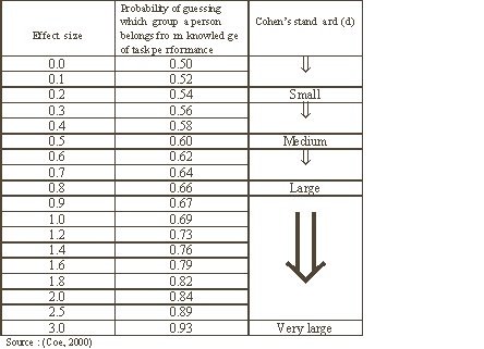
Interpreting effect sizesThere are different ways to interpret effect sizes. The table below is an adapted version of Coe (2000). For a more in depth discussion on the interpretation of effect size please refer to:
http://www.cemcentre.org/ebeuk/research/effectsize/interpret.htmTable 1. Effect size – Interpretation
Effect sizes can be converted into statements about the overlap between two groups. This can be a valuable tool when discussing the magnitude of the difference between groups. The first column in the table presents the actual effect size. The second presents the probability of guessing which group a person belongs on the basis of their performance on a specific task. If the effect size is zero than the probability of a correct guess is fifty percent. As the effect size increases, the overlap decreases and the chances of correctly identifying the group increases.
Cohen (1990; 1994) has written substantially on effect sizes and provides some guidelines for their interpretation based on the effect size of differences that are familiar. Cohen’s d is a measure of the distance between means (Denis, 2003). As noted in the table above an effect size of 0.2 is considered small and can be compared to the difference between the heights of fifteen and sixteen year old girls. An effect size of 0.5 is regarded as medium and compared to the difference in heights between fourteen and eighteen year old girls. Finally, an effect size of 0.8 is considered large and Cohen equates it to the difference in heights between thirteen and eighteen year old girls. As mentioned above effect sizes can also be reported using Hedge’s g. This is the ratio of the difference between two means divided by the combined estimate of the standard deviation.
There are no exact guidelines as to what indicates a small or large effect. Researchers should be encouraged to report both the probability value and the effect size. Reporting both values will prevent the researcher from falling in the trap of reaching significance but not knowing the strength of the relationship (magnitude of difference). Here it is important to note that effect sizes are descriptive and not inferential. They are descriptive of the sample data and offer no information on the degree of association for the rest of the population. In addition, effect sizes should be interpreted with particular care, as they are highly dependent on the situation. It is up to the investigator to become acquainted with different characteristics of the data and develop and understanding of what constitutes a small or large effect. This last recommendation should not be taken lightly especially in the behavioural sciences where a small effect can have very important implications.
Statistical significance vs. clinical significanceEffect sizes can provide information about the practical (clinical) significance of an effect. An effect can be statistically significant and mathematically real but too small to be important. For this reason it is important to differentiate between statistical and practical significance. As mentioned above, statistical significance does not provide any information about the size of an effect and is susceptible to differences in sample sizes. Trivial differences can have very low p values if the size of the sample is large enough. Practical significance is a deductive statement (judgement) about the utility of a result. It will depend on the researcher’s understanding of the situation, practical knowledge and experience. Moreover, the magnitude of an effect should not be interpreted as synonymous with practical significance. It is possible to have a small effect size that is of high practical importance and vice-versa.
Confidence intervalsRelying on information from samples of a population will always lead to some level of uncertainty. The confidence interval quantifies this uncertainty. It is a range of values within which the population parameter is likely to be included. This is calculated from the sample data and usually reported at the 95% level. In this manner, the confidence interval for the difference between to means is a range of values where the difference between the means of two populations may lie. The width of a confidence interval can provide some information about how certain we are about the difference in means. In general, the narrower the confidence interval the higher is the precision of the estimate. The confidence interval will tend to be wide when the sample size is small and the scores are less homogeneous
Confidence intervals are a useful tool for the interpretation of results and an appealing alternative to NHST given that they can also provide information as to whether the difference between two means is statistically significant. When looking at the confidence interval of a difference one can easily check whether the interval includes a value that implies “no effect”. If not stated a priori this value is usually assumed to be zero (null hypothesis).
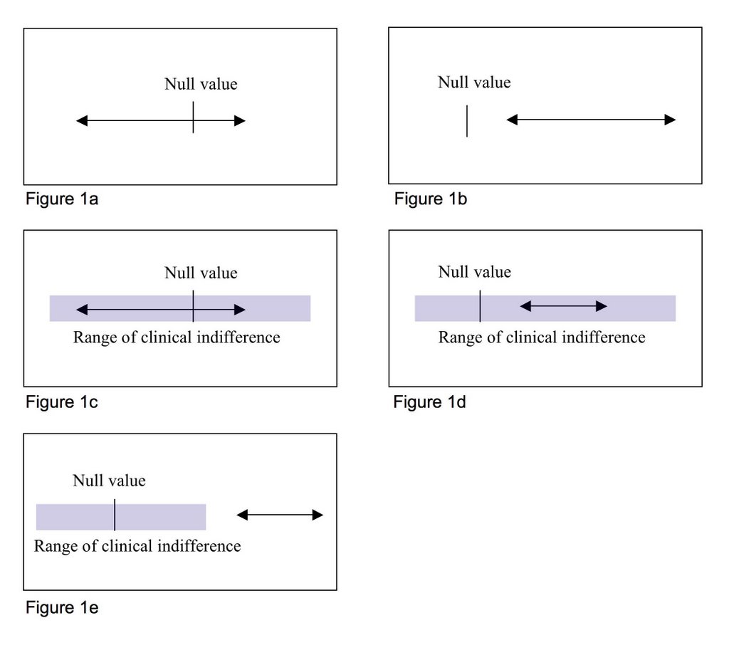
Simon (2006) provides several graphical examples as to how researcher can use confidence intervals to interpret their results. Figure 1a is an example of a confidence interval that includes the null value. In his case, the mean difference is not statistically significant. Figure 1b is an example of statistically significant difference where the null value falls outside the limits of the confidence interval. Confidence intervals also allow the researcher to interpret whether a difference is clinically significant. As mentioned above a difference can be statistically significant but of no practical value if falls within the range of clinical indifference. Figure 1c illustrates a situation in which the confidence interval includes the null value and these fall within the range of clinical indifference. Here the mean difference is neither statistically or clinically significant. In figure 1d the mean difference is statistically significant but of no clinical value given that the range of clinical indifference covers the totality of the confidence interval. Finally, figure 1e is an example of statistically and clinically significant difference where the null value lies outside the confidence interval and these lie outside the range of clinical indifference.
Figure 1 – Confidence interval and null hypothesis
 Adapted from: Steve Simon's Statisitical evidence in medical trials (pages 142-143).
Graphic representation and the initial examination of data
More effort should be put during the initial examination of data. Before engaging in statistical tests, researchers need to clarify the general structure and quality of the collected data and check for consistency, credibility and completeness (Chatfield, 1985). This can easily be achieved through descriptive statistics and graphical techniques but must also be complemented by the researcher’s experience during the data collection period. This type of data management will allow the researcher to consider not only the original hypotheses but an array of new and unlikely possibilities. Wainer & Thissen (1993) put forward some benefits of displaying data graphically:
1. Descriptive capacity: variety of description that can be simultaneously grasped
2. Versatility: Illustrate aspects of the data that were not expected
3. Data orientation: Trends and the characteristic distribution of the data
4. Potential for internal comparisons: Allows for quick comparisons within and between different data sets
5. Summary of large data: Graphs are particularly useful for summarizing large data sets
Descriptive statistics can prevent a variety of errors associated with the type of the distribution of the data. The mean can be an efficient estimate of central tendency if the population distribution is normal. However, even a slight variation in the distribution can have a large effect on the mean. In situations where the distribution is not normal, the median is a more robust measure (Smith & Prentice, 1993). Stem and leaf displays are a quick and effective way to present the shape of the distribution from particular data and check for outliers. They can also present important information about order statistics.
The “five number” summary of a data set consist of the minimum, the maximum, lower quartile, the median, the upper quartile and the maximum. It is essential for the researcher to know and report these values along with the standard deviations. A box plot is a visual display of the “five number” summary. They are particularly useful when viewed side by side and used to compare data from different groups (Tukey, 1977). The median is the line that runs across the box. The box itself stretches from the lower hinge (25th percentile) to the upper hinge (75th percentile). The lines that stretch out of the box are known as whiskers and they indicate the minimum and maximum data values. Points located beyond the whiskers (on either side) are the outliers. If the median line is not equidistant from both hinges the distribution is skewed. In a positive (right) skewed distribution the mean is larger than the median. In a negative (left) skewed distribution the mean is smaller than the median.
A good knowledge about the characteristics of a distribution can also inform the researcher about the value of the test conducted. A linear regression examines the relationship (or degree of fit) between two ordered variables. A scatter plot is usually constructed in order to visualise the data. This will allow the researcher to determine the appropriateness of the linear model and detect any departure from linearity (Smith & Prentice, 1993). In a least square regression a line is plotted where the sum of the squared distance of the points is a minimum. However, in a least square regression (the most commonly used method) an outlier can have a strong impact in the final result of the regression.
The median-to-median line (or resistant line) is a line through the data that is least affected by outliers and is an attractive alternative to the least square regression. In the resistance line technique no single point on the sample has a special influence on the projection of the line. Details for the calculation of resistant lines can be found in Velleman & Hoaglin (1981). Finally, there are several diagnostic tools for the evaluation of the adequacy of regression models (leverage, Cook’s distance, residual) and these are included in most statistical packages. Reporting Cook’s distance is particularly useful as it provides an index of the actual influence of each case on the regression function.